A new theoretical base for intracranial brain volume normalization in neuroimaging studies

In the volumetric studies of the brain, there are often conflicting results due to the presence of confounding factors such as age and gender, and covariates like brain volume. At times, in comparison with a control group, for example, this large variability is enough to confound any effect due to the pathology. For this reason, data are generally corrected or normalized by empirical methods as found in other fields of brain studies. In this study, we proposed a normalization method based on a theoretical approach. This method, based on a simple geometrical brain model, has been tested by a comparison with the empirical ones in 16 brain regions, considering two samples of subjects: 19 dyslexics and 10 healthy controls. The results show a good and interesting agreement between data and model and give a new basis for the single subject brain volume normalization. In particular, it is possible to show how the amygdala and the whole brain volume should be thought of, as linked by shape and physiological relation due to the ratio between their volumes.

Introduction

In the volumetric Magnetic Resonance Imaging (MRI) studies it is very difficult to compare the volumes of brain areas between groups of subjects because the mean differences are often small and dependent on spurious variables. Generally, the pathology of patients and the brain area volume differences are linked as cause and effect, other variables, such as age, gender and education could mask this relation, and for this reason, are usually considered confounding factors (or bias). However, the weight of the confounding factors could be eliminated or reduced, with a better selection of the studied cohort or could be evaluated with statistical methods, as done in the neurology studies of normative data [1,2].

Another variable that influences the volume of the brain’s areas is the Intracranial Volume (ICV), defined as the intracranial volume within the whole cranium, i.e. the sum of the brain and cerebellar parenchymal and vessels volume and cerebrospinal fluid [3,4]. In particular, the volume and the surface of the brain areas linearly and significantly depend on the size of the ICV [5,6]. In this context, the ICV can be considered a covariate, i.e. a variable that changes predictably and can be used to predict the effect studied. In practice, the weight of the covariate on the mean difference of brain area volume should be considered if predictable or eliminated, or attenuated, if not. For this reason, mathematical methods exist to try to remove the dependence from the ICV using empirical rules (normalization methods), because there is no way, so far, of predicting its influence on the volume of brain cortical areas. Some of these methods were compared, such as the methods of proportional, residual and covariate approaches [7,8]. The proportional approach uses the brain area volume/ICV ratios instead of the brain area volume raw data, without any particular justification other than that the two volumes are linearly dependent. The residual approach eliminates the ICV variability considering how much each patient’s brain area volume is different from that corresponding to the patient with mean ICV. The covariate approach is used in volumetric analysis software estimating the plastic deformation of the brain volume, to adapt it to a reference brain (template) in the voxel-based package Statistical Parametric Map [9], as well as in the packages that do not provide this deformation and based on the surface based analysis [10,11]. In this software, the dependence of a brain area volume (or cortical volume) from the ICV is evaluated by a linear regression analysis for each group, which determines the intercept and the slope of the regression line. Statistical tests of significance on the difference between groups are successively based on those data. In slope comparison, practically, the within-group mean volume of a given cortical area is divided by the within-group ICV; this ratio is then compared to the value derived from another group. Even if correct, this procedure reduces the statistical precision in the between-group comparison, because of the potential presence of patients with ICV varying in a wide range. Therefore, the mean value does not well represent such values. However, the empirical methods are not very satisfactory, and there is not, currently, a widely accepted method [7]. Moreover, the segmentation techniques of the brain’s areas cause further variability, in particular in the analysis of subcortical areas [12-14]. Thus, there are often conflicting results in the literature. For example, in the amygdala volumetric study [15] the results range between ‘Reduction in bilateral amygdala volume’ and ‘Enlargement in bilateral amygdala volume’. While in the corpus callosum volumetric study [16] the results range between ‘Reduction in corpus callosum volume’ and ‘NO differences in volume’.

We propose a method of comparison between homologous cortical areas among different subjects based on the evaluation of the solid angle subtended by these areas because this method is independent of variations in cerebral volume.

The main aim of this study is to show an equation, derived from a geometrical model of the brain, for predicting how the ICV affects the volume of the brain’s cortical and subcortical areas, and to prove its effectiveness in the data analysis of the brain’s volume. To this end, we compare different normalization methods, some empirical and some proposed by the model, to study which is the best to obtain the differences between the volumes of the brain’s areas in two subject groups: the control group and the dyslexic patients. Since dyslexia is considered to derive from a mild but specific alteration in brain physiology [17-19], this method turns out to be a sensitive tool to compare normalization procedures. Moreover, with the validation of the proposed model, it is possible to observe the volumetric relation between different brain areas from a new viewpoint.

Materials and methods

In this study, we included children, both boys and girls, who were diagnosed with a Specific Learning Disorder between 1 January 2007 and 31 December 2012 at the Child Neuropsychiatry and Developmental Department of the Local Health Unit 2 Umbria. The study has been approved by the Ethics Committee for health public companies in Umbria. A total of 19 dyslexic patients (14 males and 5 females) were considered, with the mean age ± SD = 12.1 ± 2.3 years, range = 9 years - 18 years. In addition, a control group of 10 healthy subjects (4 males and 6 females) age-matched (p = 0.84) was evaluated, with mean age ± SD = 11.7 ± 1.7 years, range = 9 years - 15 years. In the dyslexic group, Specific Learning Disorder diagnoses were made through psychometric tests. Initially, a cognitive test was performed: the Wechsler scale WISC-III to identify a normal cognitive level (IQ > 85), and, subsequently the Sartori DDE-II and the dysorthography tests for the assessment of dyslexia were administered [20]. IQ was also investigated in the control group, with normal results (IQ > 85).

All subjects underwent MRI with tomograph Siemens Magnetom Verio using 3 Tesla magnetic field, acquiring a sequence MPRAGE volumetric Gradient-echo T1 weighted with high contrast between grey and white matter with the following characteristics: 176 sagittal images, isotropic voxel of 1 mm³, TE = 1900 ms, TR = 2.52 ms, IT = 900 ms, flip angle = 9°, Transmitting coil: Body, FOV = 250 mm. The MRI exam of all subjects was performed after obtaining valid informed consent from the parents of both the patients and the controls.

The images in T1 were post-processed with the software Freesurfer (Martinos Center for Biomedical Imaging) following the protocol for group comparison [9,10,21], obtaining the automatic segmentation and the evaluation of volume, thickness, and cortical surface of 74 cortical areas and ICV as defined in aparc.a2009s.volume.stats3 and 9 volumes of subcortical areas as defined in aseg.volum.stats3 files, for both hemispheres of each subject. Automatic segmentation was rechecked by a neuroradiologist.

16 segmented areas, related to the pathology and the networks of language and processing of emotions [17] were selected out of a total of 83 to perform the statistical analysis. The areas considered for the study were: inferior frontal gyrus pars opercularis, orbitalis and triangularis, superior frontal gyrus, superior temporal gyrus, frontal cingulum, superior temporal gyrus temporal planum, middle temporal gyrus, temporal pole, middle occipital gyrus, inferior parietal and supramarginal angular gyrus, entorhinal and parahippocampal cortex, cerebellar cortex and amygdala.

The statistical analysis included only the 16 selected areas and the data of cortical volumes as shown in the previously mentioned files produced by the Freesurfer software.

The data were analyzed in two different ways. Initially, a linear regression study was performed on the whole group of subjects (dyslexics + controls) to verify, for the selected cortical areas, the relationship between cortical volumes and ICV. This study has allowed for a definition of the theoretical model, discussed in the results, using a more representative sample.

Subsequently, a comparison test (unpaired t-test) was conducted between groups on the data, dyslexic versus controls, to highlight areas where the volume differences were statistically significant (p < 0.05). The tests were repeated on the volumes of the considered areas in the right and left hemispheres and on the average value. The tests were conducted by normalizing the volume data according to four different procedures to allow for a comparison between each standardization procedure and to identify the best way to discriminate significantly different areas between the two groups.

For this purpose, the criterion used was the evaluation of the decrease in the p-value of the Student-T test. By definition, the p-value represents the probability of obtaining experimental data as extreme as, or more extreme than the experimental data, once the null hypothesis is assumed to be true. Specifically, our null hypothesis was that the volume of the cortical area in the dyslexic group and the control group was the same. Moreover, in the Student-T test between the two groups, the P-value depends (both inversely) on the sample size and on the effect size (a measure of distance between the distributions of the two groups, expressed as the ratio between the difference of the two means and the standard deviation). In the comparison of different normalizations for a chosen area, both these variables are fixed and a decrease in P-value could note a better elaboration of the experimental data [22-25]. Normalization tests were as follows, for both the right and left hemisphere areas:

1. No normalization: cortical and subcortical volumes considered absolute volumes (frequently used approach)
2. Cortical and subcortical volumes were divided by the subject’s ICV (proportional approach and our model-based approximated approach).
3. Cortical and sub-cortical volumes were fitted first using the linear regression line against the ICV (group by group) and then the slopes of the straight line were compared between the two groups to check if statistically significant differences appeared (covariate approach). This data processing was carried out using the MINITAB 17 software package that allows to evaluation of the significance of the regression line in each group and the whole data set (dyslexics and controls) as well as the significance of the difference between the slopes of the regression lines between the two groups. This normalization procedure is similar to that shown in the volumetric analysis software tools such as those used in spam for Voxel-Based Morphometry (VBM) or automatic segmentation as in free surfer.
4. Cortical and sub-cortical volumes were divided by the ratio between ICV and the radius of the brain of the subject (our model-based approach). The brain radius was calculated assuming the brain was a sphere with the same volume (ICV).

Results and discussions

The proposed geometrical model and its application in the ‘all subjects analysis’

Geometrical model: A simple model for the study of volumes of different brain areas and their proportions was developed in this work. This model attempts to interpret the experimental data presented and to create quantitative relations between the observations. The basic idea of the model is to consider the brain as a sphere, even if it is not generally true. This strong choice can find a justification considering that it is always possible to approximate a brain with a sphere once a geometric topological transformation, connecting the brain to a sphere (and vice versa), can be found. The same type of transformation is used for example in the so-called cerebral cortex ‘inflated’ representation [26]. This method, in which the cortical areas are represented as exposed to the outer surface, is considered ‘smooth’ and differentiable, which recalls the surface of the cerebral hemispheres, including the areas generally hidden located in the grooves of the convolutions. The brain, during the topological transformation described, can be visually depicted as a balloon in which we blow air so that all the cortical invaginations emerge.

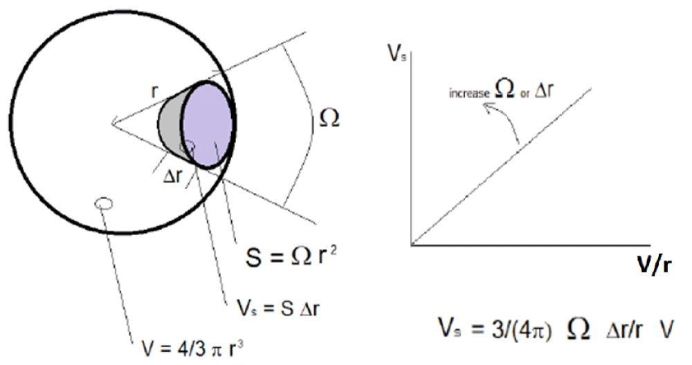
The radius r can define a sphere with volume V as the volume of a brain. The cerebral cortex can be represented as the external layer Δr<< r of the sphere. For each cortical area s with volume Vs and surface S, exists a similar area on the sphere, defined by the solid angle Ω.

In a sphere:

V = 4/3 π r3 (1)

From which

r² =3/(4 π) V/r (2)

Furthermore, for a generic cortical area ‘s’ it approximately follows that:

Vs = S ∆r (3)

In addition, for the definition of solid angle:

S = Ω r² (4)

Therefore:

Vs = Ω r² ∆r (5)

From which, placing the relation (2) in (5) we have:

Vs = 3/(4 π) Ω ∆r/r V (6)

As a consequence of the relation (6), the volume Vs of a single cortical area is linearly dependent on the solid angle Ω and the thickness Δr (local variables). In addition, the geometry, and the size, of the sphere are described by the parameter V/r (global variables). Accordingly, in (6), the ‘local’ contributions from the cortex are emphasized in comparison with the ‘global’ contributions coming from the whole brain once the solid angle Ω, defining the projection of a single cortical area, is independent of the whole brain volume. By contrast, the same relation is not valid in (3), since it only allows us to define Vs by its area S, which is strictly related to the whole brain volume. Therefore, as suggested by (6), the normalization of Vs to the ratio V/r eliminates the dependence of Vs on the size of the sphere (size of the brain). Nevertheless, the normalization to the single volume V represents a good alternative method, as shown after. Finally, it should be noted that, for a sphere, the Δr/r ratio is independent of r, because we might suppose Δr as a first-order differential of r. In fact, under this assumption, Δr is proportional to r, and the ratio Δr/r is independent of r. unfortunately, this assumption is not valid in the case of the brain where cortical thickness is independent from the radius of the brain, as proven by the data reported in the next paragraph. For this reason, (6) can be reshaped as follows by applying it to the anatomical case:

Vs = 3/(4 π) Ω ∆t/r V (7)

With ∆t equal to cortical thickness. The relation (6) is graphically depicted in Figure 1. A consequence of (7) is that, under this model, the effect of a pathology that changes some of the brain area volumes between two groups of subjects, even if present in some mean ICV difference (V/r), could be due, separately and independently only to: the mean size (Ω) and the mean thickness (∆t). In practice, the Vs/(V/r) ratios (i.e. for the relation of r to V, Vs/(4 π V2/3)1/3) produce data that is independent of global brain size variability.

Figure 1: On the left, a spherical calotte is depicted, where, the thickness, indicated by ∆r (∆r<< r), the solid angle by Ω, and the spherical surface of the calotte by S, allow us to calculate the calotte volume Vs like in the equation on the right. The equation on the right, and the diagram shows that the volume Vs of the truncated cone is linearly dependent on the ratio V/r, where V and r represent the ‘global variables’. While V and rare characteristics of the whole sphere, Ω and Δr represent the ‘local variables’ describing the single cortical area. In addition, the slope of the linear dependence of Vs by V/r increases when the product Ω Δr increases.

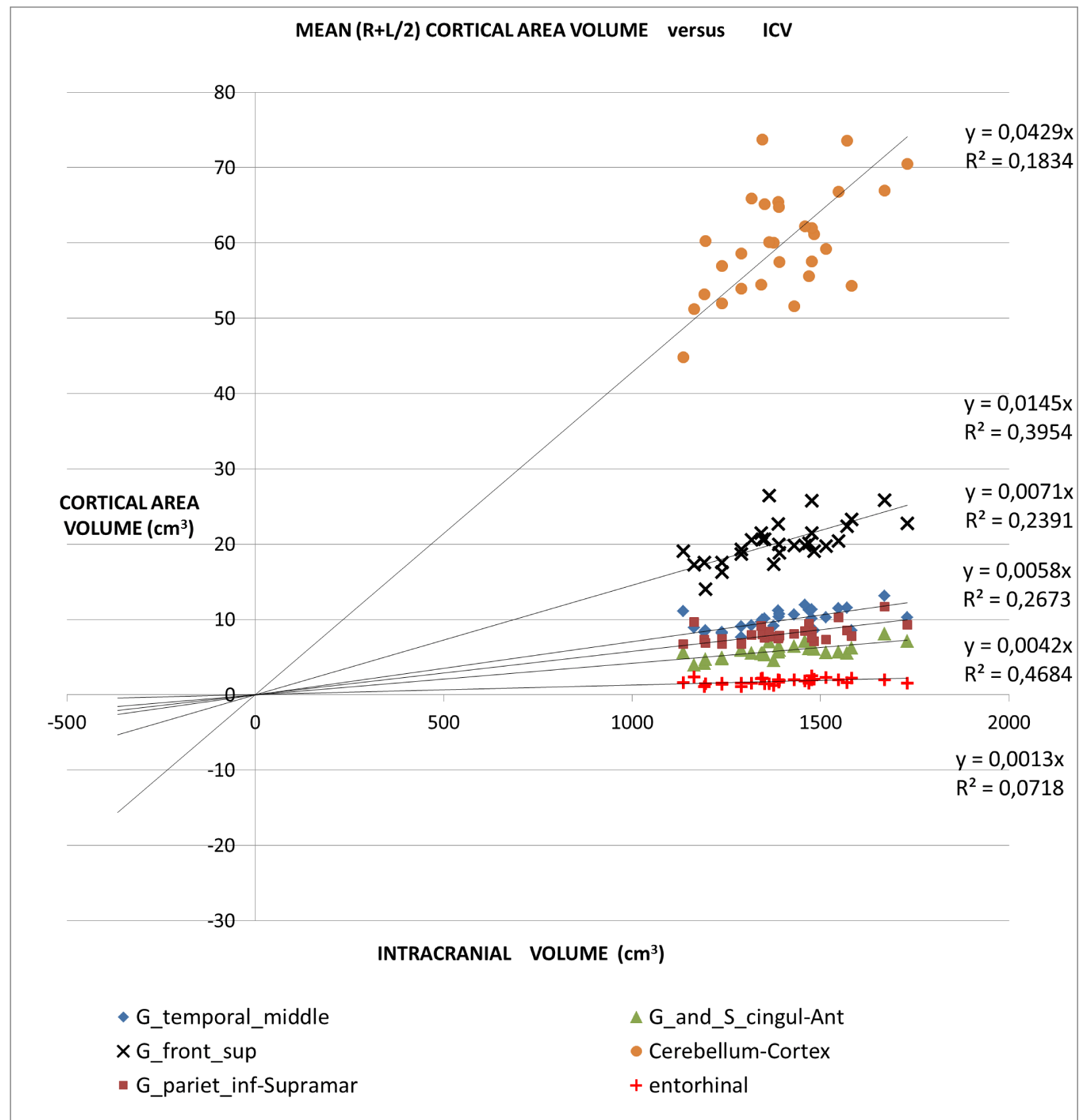
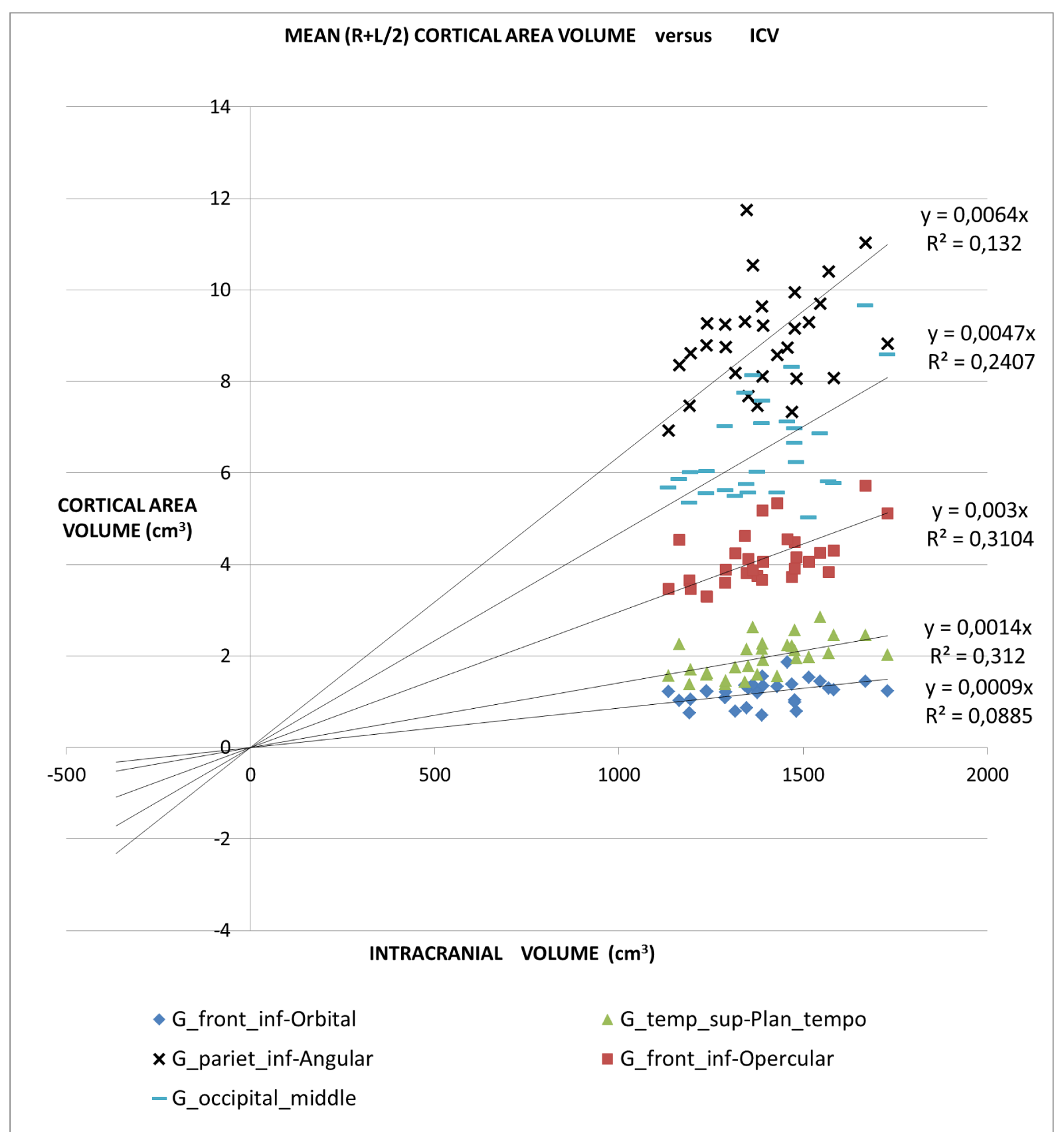
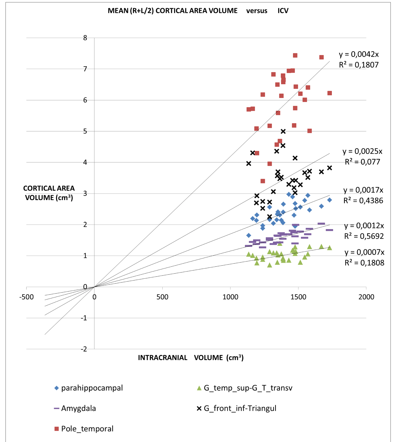
An application of this model is presented in Figures 2A,2B and 2C in which different brain areas are regrouped under different solid angle sizes (i.e. different slopes of straight lines). In all this data we could hypothesize that the thickness does not depend on the V/r ratio (∆t≈constant). In fact, from our data, the mean (left-right) thickness over the whole 16 areas varies between subjects in the range 2,7 and 3,2 mm (mean ± sd = (2.9 ± 0.1)mm) and the correspondent variation coefficients in the range 11% - 18%. Furthermore, the linear regression between the mean brain thickness (y) and the brain volume(x) is not a significant straight line with a very low slope (y = -0.0002x +3.18; R² = 0,0486; R²(limit 5%, 14 fd) = 0.264). The T-tests for thickness differences between the two groups are not significant, over the 16 brain areas.

Figure 2A:

Figure 2B:

For all the brain areas in Figure 2A-C, a regression test for the volume dependence by the subject’s age and gender was checked, with no significant results.

Figure 2C: Figures 2A, 2B, and 2C show the mean of the right and left hemisphere volumes of 16 cortical and subcortical areas to the subject’s intracranial volume for the whole group of subjects (19 dyslexics and 10 controls). These data were obtained from the Freesurfer’s file aparc.a2009s.volume.stats3 e aseg.volum.stats3. The best linear fits, the relative equations, and the corresponding value of the regression coefficient are also shown. The regressions are considered significant when R² ≥ 0,1369 (p ≤ 0.05). These graphs show that the larger the (mean) cortical (or sub-cortical) area is, the higher the slope of the regression line results, as predicted by equation (7) in the text. Since the differences between the two groups are, generally, not significant, they are not shown in the figures.

All subjects analysis: A linear regression study

Table 1 presents in numerical form the results shown in Figures 2A, 2B, and 2C.

Different normalizations comparison: The ‘between subjects’ analysis

Table 2 data shows that for the amygdala, a redundant and significant statistical certainty that between the dyslexics and the control group, a difference in the volume of this brain area exists, regardless of the hemisphere considered (or their mean) but not for the normalization approach. This difference is significant only from the B and D-type normalizations.

The B and D type normalizations highlighted even the differences in the left hemisphere for the superior temporal gyrus – planum temporale (area 7).

The C-type normalizations highlighted significant differences in the left hemisphere in areas 8 and 11, and areas 5 and 12 on the right.

A geometric model is proposed in this article, and an equation describing the relationship between the volume of brain areas and the volume of the whole brain. The effectiveness of the descriptive capacity of the proposed model is expressed and verified by the following considerations.

‘all subjects analysis’: In this study, we proposed a normalization method based on a theoretical approach. In the normal brain, volume brain areas increase with volume, but at a different rate. The bigger ones increased more than the smaller ones. Considering data from 16 brain regions of normal subjects our model shows the same trend.

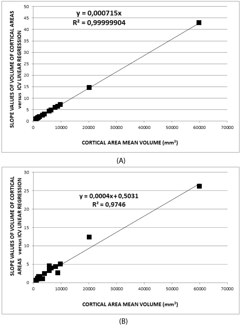
The all-subject analysis shows systematically (Figures 2A-C), that the bigger the (mean) cortical (or sub-cortical) volume the higher the slope of the regression line. The result persists even when the data are fitted with a regression line with a non-zero intercept. The cortical areas that are worst represented by the linear model are those with a strong lateralization of the function specifically the inferior parietal angular gyrus (R² = 0.132) and triangular inferior frontal gyrus (R² = 0.077). For such areas, the average value between the right and left hemispheres is not appropriate.

Figures 3A and 3B allow some additional observations compared to what was shown in Figures 2A, 2B, and 2C.

Figure 3A,B: Figures 3A and 3B show the values of the slopes of the regression lines of Figures 2A, 2B, and 2C plotted as a function of the average volume of the 16 considered areas (average value on all the 29 subjects) when the intercepts are fixed to zero (3A) or are left as a free parameter of the linear fit (3B), respectively.

- Quantitatively, the higher the average volume of the cortical areas is, the higher the slopes of the best linear fit are, but this significant relation is linear, as predicted in the proposed model (R²(limit 5%, 14 f.d.)=0.264).

- The linear relationship includes cortical areas with a wide range of average volume and located in different brain regions. The minimum average cortical volume is in the superior temporal gyrus (average size of about 1000 mm³) and the maximum is in the cerebellar cortex (average volume of about 60000 mm³).

- When the fit is performed with the intercept as a free parameter, the regression coefficient is lower than the case of the fit with the intercept fixed to zero (lower freedom degree). Inversely due to statistical reasons, but conformably concerning the proposed model. It is possible to justify this choice also with a second consideration.

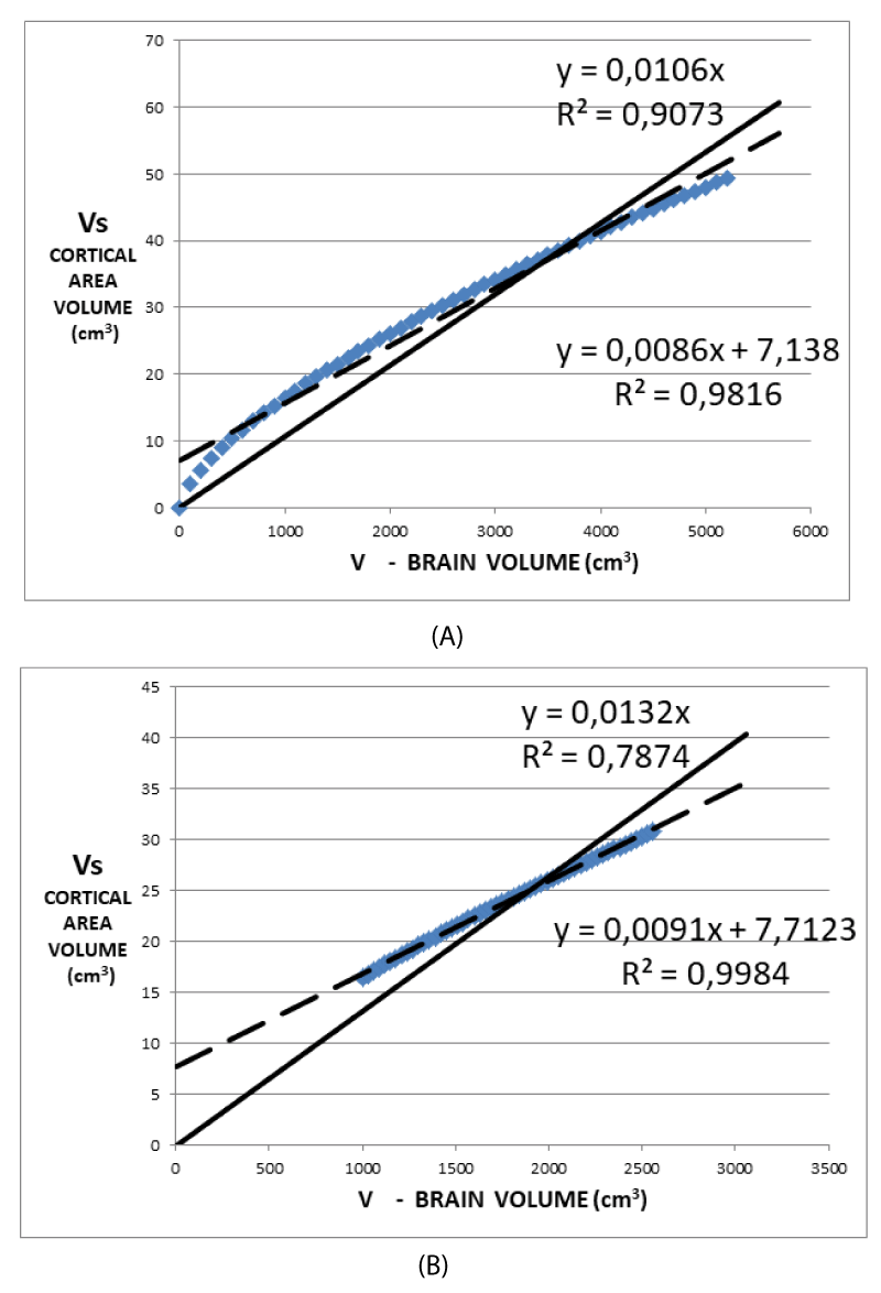
Figures 4A and 4B graphically show the (7). In (7) Vs is expressed as a function of V once the values of Ω, ∆t are assumed as 1.22 steradians, 3.5 mm respectively, while r is deduced by V by making use of (1). These data are the result of the data analysis of a superior frontal cortical area of the first control. Figure 4A shows the values of Vs as deduced from (7) for a range of values of V much wider than that of the physiological values. Figure 4B shows more realistic values V ranging around values considered physiological for subjects in the age range of 8 - 10 years. Both of these figures show that a regression line with a non-zero intercept, generally used in the analysis of data derived from images, better approximates the (7) when a linear regression is performed. Conversely, the (7) assumes an intercept value of zero. Consequently, reproducing the experimental data with a regression line provided with a non-zero intercept systematically introduces an error. This is the basic reason for using zero as the intercept value of the model, as shown in Figures 2A, 2B, and 2C. A comparison of Figures 3A and 3B clearly shows the introduction of a systematic error in the data analysis. Noteworthy, is the factor 1/r in (7) which is not compatible with a perfectly straight line in the simulations shown in Figures 4A and 4B. For this reason, the normalization of Vs by V does not eliminate the dependence on the size of the brain due to the factor 1/r but represents a good compromise. Plotting as a function of V/r would show a linear behavior in Figures 4A and 4B. Once normalization to the volume V is applied, a maximum difference of 2% is obtained when the non-zero intercept is assumed, while the maximum difference rises to 24% in the case of zero intercept.

Figure 4A,B: Figures 4A and 4B show (blue dots) the equation (7): Vs = 3/(4 π) Ω ∆t/r V, as described in the text, in which the volume Vs of a cortical brain area, underlying a solid angle Ω and with thickness ∆t (respectively for the frontal superior gyrus area of the control n.1 equal to 1.22 steradians and 3.5 mm), is calculated for a range of brain volumes V wider than (4A) or ranging around (4B) physiological values of subjects around 8 and 10 years old. In addition, the Figure shows the regression lines in which the intercept is a free parameter (dashed line) or is fixed to zero (whole line). It is possible to note that the Vs values follow a curve line due to the 1/r influences (r is the radius of a sphere with the same brain volume V). This feature is even more evident in 4A. Furthermore, the use of the not zero intercept regression (dotted line), as currently used in literature, leads to a better fit, but this is paid for by the introduction of a confounding term (and a systematic error) not provided by the (7).

The main information in (7) is that it accurately describes the data derived from the images and the automatic segmentation of individual cortical areas through the Freesurfer software. The (7) predicts that:

1. In a Vs against V graph, the slope grows linearly with the solid angle Ω, once the cortical thickness is assumed approximately constant. This trend is visible both in the graphs shown in Figures 2A-2C as well as in Figure 3A, where it is resumed in a single graph. A large enough spread in the brain’s volumes, as in our case, is necessary to test and graphically reproduce such a trend on other series (groups of patients and/or controls). The (7) addresses the difference between a group with a pathology and a healthy one to two possible causes once the V volume is not linked to the disease, that is Ω and ∆t.
2. The normalized values of Vs by V (subject by subject), still show a slight dependence on the value of V. The literature shows several examples of a slightly decreasing linear trend of Vs/V as a function of V. From a quantitative point of view:

Vs/V = 3/(4 π) Ω ∆t/r (8)

And by placing the value of r that deducted by (1) you have:

Vs/V = 3/(4 π) Ω ∆t/[3V/(4 π)]^1/3 (9)

The (9) is a weakly decreasing function concerning V. The (9) implicitly explains the values in t Table 1 column 6, showing negative data to all the entries except just two values. Numerically, making use of the simulated data, the slope of the (9) is about -3E-6 while in Table 1 there is an average value of about -1.4E-3.

3. The (7) provides that, as shown in Figures 4A and 4B, fitting Vs as a function of V with null intercept, leads to an overestimation of the slope values compared to the non-zero intercept case. This result is in agreement with the experimental data reported in the fourth and fifth columns of Table 1. From the simulation data in Table 1, the percentage difference between the two slopes is about 45%, similar to the difference between the mean values of column 4 and column 5 of Table 1 (46.5%).

‘Between subjects analysis’: The results and the data analysis of this work show that the B- and D-type normalizations are more reliable than C from a clinical point of view. In addition, such methods can distinguish the two groups of data more significantly as shown in Table 3A-C with an elaboration of results reported in Table 2 and the following considerations.

Considering the reduction of the p - value on the highest number of cortical areas, such as the criterion used to perform the comparison between normalizations, we see that:

It is generally necessary to normalize the data. Regardless of the analysis being carried out on one or both (mean values) of the hemispheres, the three normalizations (B, C, and D) proposed, determine the decrease of the p - values in some areas and the increase in others. The percentage of decreased p-values ranges between twice and three times the percentage of increased p - values (Tables 3A-C).

The B-type standardization gives better results than the C- and D-type. Similar results as highlighted in the preceding point, are obtained by comparing the B-type normalization with C- and D-type.

The choice of normalization strongly determines the areas with significant results. As a consequence, the normalization used has a strong clinical impact.

It is generally necessary to make separate assessments for each hemisphere. Considering the area n° 7 (Table 2) as an example, in the superior temporal gyrus - temporal planum, the difference between the volumes of the two groups is significant with both the B- and D-type normalizations only on the left hemisphere. Numerically, applying normalization of type A, the average volume ± sd of 7SIN area in the controls is (1980 ± 420) cm3, while, in dyslexics, it is (2270 ± 520) cm3 (p = 0.117, standard difference = 0.58). When the normalization of B-type is in use, the average volume ± sd of 7SIN area is (1.39 ± 0.2) arbitrary unit (a.u.) and (1.64 ± 0.35) a.u. for the controls and the dyslexics respectively (p = 0.022, standard difference = 0.77). Applying the D-type normalization, the 7SIN average volume ± sd is (9.7 ± 1.6) cm and (11.3 ± 2.4) cm for the control group and the dyslexic respectively (p = 0.038, standard difference = 0.72).

It is possible to show that significant differences highlighted for the C-type normalization, albeit significant, are due to the statistical instability of the regression line (outlier data) used to fit the data and don’t have clinical meaning as shown in more detail in the Appendix.

In summary, B- and D-type normalizations work better concerning C- and A-type because B- and D-type are based on a geometric descriptive model. The model takes into account the volumetry of the brain both as a whole organ and as an assembly of its parts. In addition, it is worth noting that the fit in Figure 3A has a regression coefficient of 0.9999904, which demonstrates a strong linear relation. Furthermore, (7) determines the relationships of scale between volumes of the individual areas and the whole brain which vary from subject to subject. The common analysis, using the average values in the groups, hides the differences between brains in the sample, giving results less sensible to the single subject characteristics. In addition, the outliers have influences on the average values as well as the fit goodness, as represented in the Appendix. As a consequence, assuming that this model represents the truth, it follows that in brain volumetric studies, it is necessary to normalize the volume of any cortical or subcortical brain area before performing group analysis. Therefore, these relationships must be taken into account. In addition, (7) gives a completely different meaning to the covariate effect linked to brain volume. Some considerations follow:

- The (7) describes the most simple geometrical model of the brain among a class of similar models.

- The (7) applied to the whole brain leads to a total solid angle of about 2.6 times that of a sphere. This implies that (7) takes account of the external surfaces of the cortical areas that can contain invaginations due to the shape of the convolutions.

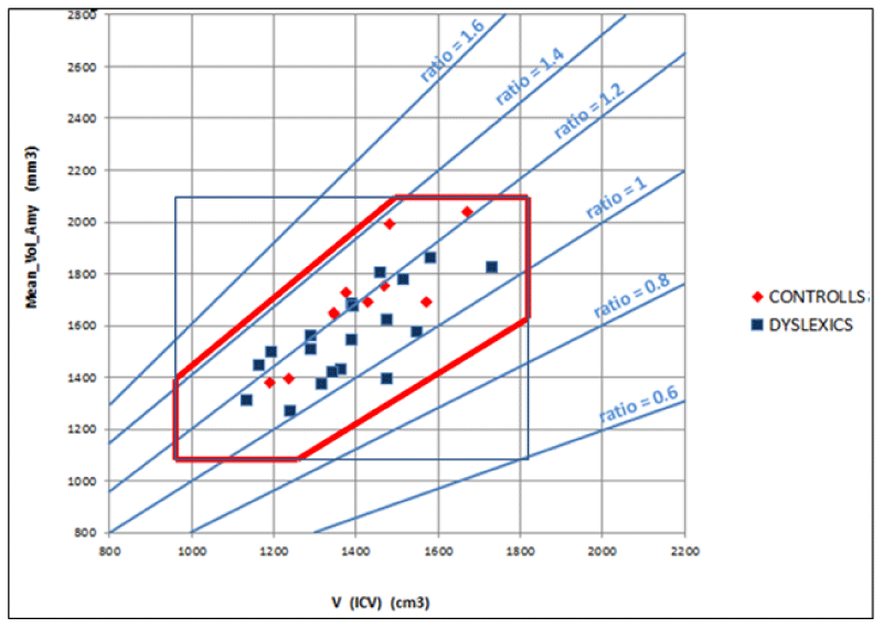
- The (7), coming from a geometrical model of the brain, relates the characteristics of cortical areas with each other in the brain. Particularly, the volumes of the different cortical areas in healthy subjects seem not to be independent of each other and the whole brain volume. To be clearer, certain dimensional relationships are respected as in another anatomical region of the human body. For example, the scapula bone size is not independent of the size of the homers bone. Seemingly, the significant regressions shown in Figure 5 imply that between amygdala volume and the volume of the whole brain the following ratio exists: in 99% (3 standard deviations) of the healthy population, the amygdala volume (sum of the volumes of the two hemispheres) is 2.3 ± 0.6 mm³ for each cm3 of the whole brain. Consequently, the ratio of the two volumes is as meaningful as or more than the absolute volumes. Figure 5 shows, for all the subjects (healthy and not), taken as a representative sample of the healthy population, the combined intervals of variability within three standard deviations, defined and identified for the volume of the whole brain and the amygdala and their ratio. This highlights that possible pathological values are detectable for alterations of the relationship between amygdala volume and whole brain volume even in the case of absolute values inside the range considered as normal.

Figure 5: The average volume of the amygdala (averaging between the left and right side volume) is plotted against intracranial volume (ICV) for all the 29 subjects considered in this article, separated between controls (red dots) and dyslexic (blue points). In addition, the lines through the origin describing relations between amygdala volume (in mm³) and ICV (in cm3) are drawn ranging from 1.6 to 0.6. Assuming the two groups are a single ensemble, it is possible to determine the range of variability to 99% (mean ± 3SD) of the average volume of the amygdala (the horizontal sides of the square in blue, 1600 ± 570 mm³), ICV (vertical sides of the square in blue, 1390 ± 430 cm3) and their relationship (oblique sides of the hexagon in red, 1.15 ± 0.30 in mm³/cm3). The triangles (upper left and bottom right), delimited by the external square described by the average values ± 3SD and the red hexagon, could contain pathological values for the ratio between amygdala volume and ICV but non-normal absolute values.

Clinical details

In this publication, given the technical approach described, the clinical aspects relating to the results for which the ratio between amygdala volume and intracranial volume is significantly smaller in the dyslexic group compared to that of normal subjects are not extensively described. Nevertheless, it is possible to speculate that difficulties in focusing in dyslexic subjects, both in visual perception and in the next steps involved in the reading process, can arise from the functions and the reduced connectivity of the amygdala which has, concerning brain volume, a small volume.

Some particular aspect

Ultimately one might ask why this proposed model should be used? The fact that it allows us to justify the use of normalization for the cerebral volume V alone, frequently used in the literature, is not in itself a justification given that the normalization which should have been more advanced (division by V/r), does not seem to give better results in the range of variation of V considered for the subjects of this publication.

So I try to outline some further reasons to underline its interest. Firstly, it has been demonstrated that it behaves as the data predict, both through the dependence of these on the brain volume as the solid angle varies, positioning cortical areas with larger volumes in areas higher up in the graph, but at the same time, always tilting the regression line that approximates them is more. Both by the presence of the not completely linear trend of equation (7) as the brain volume varies. That is, by the presence of the ‘hump’ corresponding to ICV values ​​around 50 cc, in this relationship. This, although not corroborated by real data, is shown through its direct effect on the slope of the regression lines with or without angular parameters free to vary.

Furthermore, the model is interesting as it justifies why we move, in cerebral volumetry, from the use of the volumes or surfaces of the cortical areas to the solid angle they subtend. Since this does not vary if ICV varies.

Finally, some further considerations on the use of the solid angle.

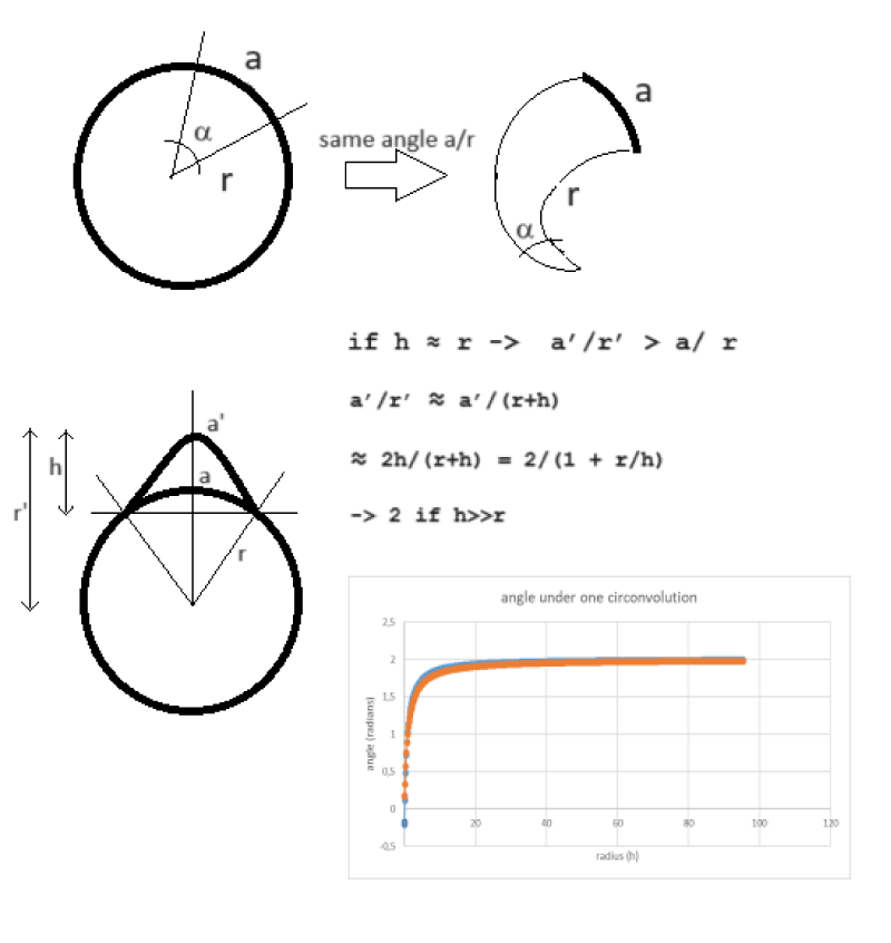
Imagine drawing a circle in the plane and delineating an angle from its center. The extension of this angle can be expressed in radians through the ratio between the length of the chord subtended on the circumference and the radius of the circumference. Let us then consider an angle of approximately one radian, such as that approximately subtended by a cerebral convolution in an axial slice of a normal human brain. The effect of the convolution is configured as that of extending the length of the subtended arc, compared to if it were a circumference, and also lengthening the length of the radius. As reported in Figure 6, it can be demonstrated that the presence of the gyrus leads to an increase in the size of the subtended angle. This growth brings the angle from 1 to a maximum of 2 radians. This can be demonstrated geometrically. So why does the proposed model hold up, compared to the geometry of a sphere from which it is inspired, despite the presence of the convolutions that alter this plane angle and consequently also the corresponding solid angle in 3D? Probably precisely because the variation in solid angle introduced by the gyrus is also independent of the brain volume. So it would seem that the most salient feature of the proposed model is, fundamentally, that expressing the cortical extensions in solid angles (steradian) rather than in volumes (cm3) or surfaces (cm2) makes us completely independent of the brain volume. At this point, we could think of further perfecting the technique by developing the geometry and considering not a single average ray for the whole brain, as supposed in that publication, but a different abscissa for each brain area that starts from a single point common to the whole brain inside the brain and extends to the middle apex of each convolution.

Figure 6: The deformations of one angle. Up: The angle alfa is the same because the a/r ratio is the same. Down: The angle subtended for deformation of arc a in to a’, increase the angle a/r (≈1 rad) till 2 rad, as exposed in the middle and the graph.

Limitations, perspectives, and recommendations

This study shows two principal limitations. First, the prevalent fenomenologic exposition. Second, the mathematical approach doesn’t contain a clear theoric topologic justification of the geometry aspect that links the cortical volume of a brain area to the correspondent on the sphere. For that, we could develop a study with a deeper clinical database validated in pathologic vs health subjects comparison to improve the statistical aspects of the work and to reduce uncertainties. Secondly, to develop a non-fenomenologic approach to the theory. For example, describing a continuum 3D topologic transformation between sphere and brain.

Appendix

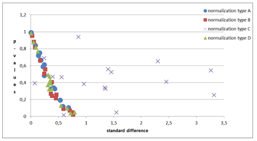
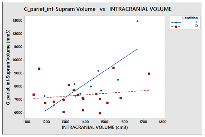
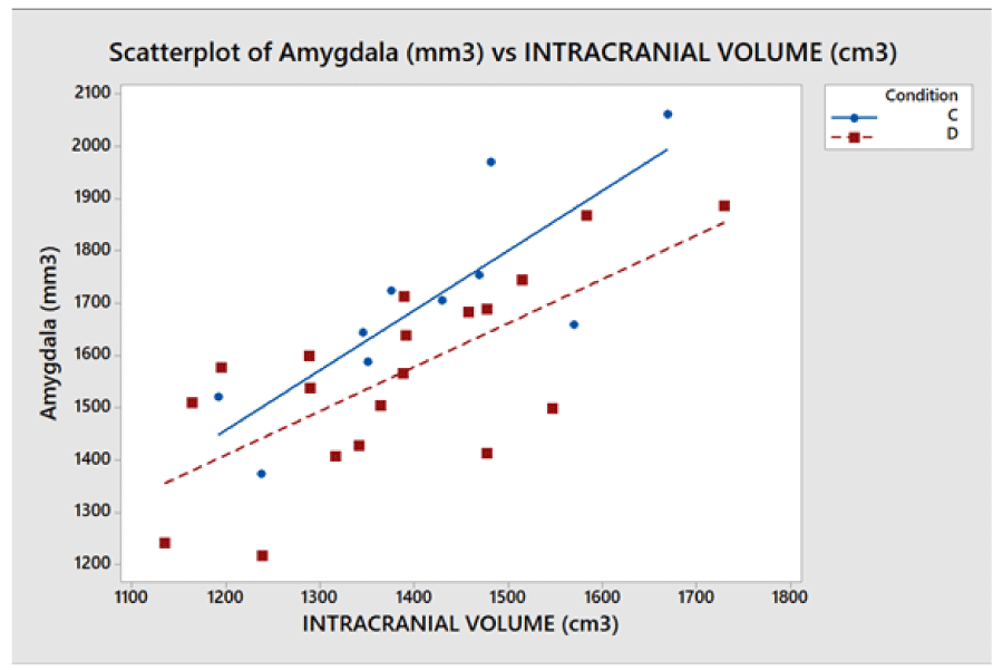
The problems of C-type normalization: The standard difference is defined here as the ratio between the absolute difference in the average volume of the cortical areas in the two groups and the standard deviation on the whole sample of subjects (dyslexic and controls). The p - value generally decreases when the standard difference increases when A-, B- and D-type normalizations are applied, as shown in the literature [23,26]. This is shown in Figure 7. By contrast the C-type standardization, based on a two-slope comparison, does not have this effect and gives different results. Such behavior can be explained as follows. For a given cortical (or subcortical) area, the regression lines are generally significant for the whole sample of 29 subjects but not for both groups, and this is because the regression lines for less numerous groups strongly depend on the noise level of the data and the presence of outliers data, but surprisingly this often produces significantly different slopes. As an example, this situation occurred (Table 2), in the areas identified by the number 5 (p = 0.028) and 12 (p = 0.006) on the right hemisphere and in areas 8 (p = 0.047) and 11 (p = 0.015) on the left. The results shown in these areas are not clinically reliable. More in detail, the analysis of the area 12 data on the right inferior parietal gyrus – supramarginal gives the following values ​​of the square regression coefficients R² and p-values on the whole group (29 subjects) of data: R² = 47.3%, p < 0.001. When the two groups are analyzed separately, R² is 64.1% and 2.7% for the Dyslexic and for the Control group respectively, while p(different_slope_C_vs_D) results < 0.006. In practice, it is clear that the R² values for the whole group and the p-value for the different slopes are driven only by one outlier data present in the Dyslexic group, as shown in Figure 8. These cannot be clinically accepted, as in the other C-type significant results. Figure 9 shows an opposite scenario when considering the right amygdala area. In this case, even if the difference between the linear regression slopes is not significant, the regression on both groups taken separately is significant. In addition, the regression is significant on the whole sample of data. The consequence is that the amygdala, regardless of the hemisphere (Table 2), is the only area showing significant redundancy between both the normalized (B and D-Type)and non-normalized data (A-Type), but not for the C-type.

Figure 7: This Figure shows an elaboration of the data in Table 1. For left hemisphere data, the p-values for the Student test between the two groups versus the standard differences defined were shown, for the selected cortical areas, as the ratio between the mean normalized volume difference between the two groups and the standard deviation of the whole subjects group (a measure of the effect size between the two populations). As shown for the normalization types A, B, and D an increased standard difference (bigger effect size) corresponds to a p – p-p-value decrease. For this reason is corrected considering better a normalization with lower p-value. The data for the C-type are noisy and follow an unusual decrease likely due to the effect on the regression line by the outliers data. The data for the right hemisphere weren’t shown because there was only one equivalent graph.

Figure 8: Scatterplot of the right Gyrus parietal inferior–supramarginal volume vs Intracranial Volume for the two groups of subjects (D-Dyslexics and C-Controls) and correspondent regression lines. We noted that despite the significant regression model for the whole group of subjects (p(regression_modell_D+C) < 0,001; R²(D+C) = 47,3%), the significant different slope (p(different_slope_C_vs_D) < 0,006) is due to only one outlier isolated data ((x,y) = 1670, 12957) and this is also described by these statistics for single groups: R²(D) = 64,1%; R²(C) = 2,7%. In practice, if the difference between slopes is tested only with the significance of the whole group regression and not for the single group, the C-type normalization results are clinically unreliable.

Figure 9: Scatterplot of the right Amygdala volume vs Intracranial Volume for the two groups of subjects (D-Dyslexics and C-Controls) and correspondent regression lines. We noted in this case the significant regression model for the whole group (p(regression_modell_D+C) < 0,0005; R²(D+C) = 61,4%) and for each group (R²(D) = 67,9%; R²(C) = 49,6%) although the different slope was insignificant (p(different_slope_C_vs_D) = 0,403). The difference between these two groups becomes significant if the data are expressed with the B and D-type normalizations. A similar trend was found in the data of the left and mean Amygdala volume.

Conclusion

In this publication, the need for the use of normalization methods of data in studies of brain volume, to take into account the variability of the volume of the whole brain, has been highlighted.

Key points

- A geometric model of brain area volume evaluation is presented. This model justifies why the normalization method of brain area volume with ICV is corrected. This model allows us to compare two different brains without considering that one is bigger than the other.

- The geometric approach is due to the use of a solid angle subtended of a cortical area and the idea that the cone of this solid angle remains unchanged also for severe distortions like it was made of foam.

Take home messages

- To compare angles solid subtended by a brain cortical area should be better than comparing the correspondent volume.

I would like to thank Dr. Alessia Mattacchioni for all the help she has given me in writing this article; she has given me precious tips, offered her strong support, and has always understood the originality of the article. 

Dr. Muti Marco

1. Capitani E. Statistical methods. In: Spinnler H, Tognoni G (eds) Standardizzazione e taratura di test neuropsicologici [Italian normative values and standardization of neuropsychological tests]. Ital J Neurol Sci. 1987; 6(Suppl 8):14-20.
2. Luzzi S, Pesallaccia M, Fabi K, Muti M, Viticchi G, Provinciali L, Piccirilli M. Non-verbal memory measured by Rey-Osterrieth Complex Figure B: normative data. Neurol Sci. 2011 Dec; 32(6):1081-9. doi: 10.1007/s10072-011-0641-1. Epub 2011 Jun 1. PMID: 21630034.
3. Sanfilipo MP, Benedict RH, Zivadinov R, Bakshi R. Correction for intracranial volume in analysis of whole brain atrophy in multiple sclerosis: the proportion vs. residual method. Neuroimage. 2004 Aug; 22(4):1732-43. doi: 10.1016/j.neuroimage.2004.03.037. PMID: 15275929.
4. Arndt S, Cohen G, Alliger RJ, Swayze VW 2nd, Andreasen NC. Problems with ratio and proportion measures of imaged cerebral structures. Psychiatry Res. 1991 May; 40(1):79-89. doi: 10.1016/0925-4927(91)90031-k. PMID: 1946842.
5. Barnes J, Ridgway GR, Bartlett J, Henley SM, Lehmann M, Hobbs N, Clarkson MJ, MacManus DG, Ourselin S, Fox NC. Head size, age and gender adjustment in MRI studies: a necessary nuisance? Neuroimage. 2010 Dec; 53(4):1244-55. doi: 10.1016/j.neuroimage.2010.06.025. Epub 2010 Jun 16. PMID: 20600995.
6. Nordenskjöld R, Malmberg F, Larsson EM, Simmons A, Ahlström H, Johansson L, Kullberg J. Intracranial volume normalization methods: considerations when investigating gender differences in regional brain volume. Psychiatry Res. 2015 Mar 30; 231(3):227-35. doi: 10.1016/j.pscychresns.2014.11.011. Epub 2014 Dec 5. PMID: 25665840.
7. O'Brien LM, Ziegler DA, Deutsch CK, Frazier JA, Herbert MR, Locascio JJ. Statistical adjustments for brain size in volumetric neuroimaging studies: some practical implications in methods. Psychiatry Res. 2011 Aug 30; 193(2):113-22. doi: 10.1016/j.pscychresns.2011.01.007. PMID: 21684724; PMCID: PMC3510982.
8. Voevodskaya O, Simmons A, Nordenskjöld R, Kullberg J, Ahlström H, Lind L, Wahlund LO, Larsson EM, Westman E; Alzheimer's Disease Neuroimaging Initiative. The effects of intracranial volume adjustment approaches on multiple regional MRI volumes in healthy aging and Alzheimer's disease. Front Aging Neurosci. 2014 Oct 7; 6:264. doi: 10.3389/fnagi.2014.00264. PMID: 25339897; PMCID: PMC4188138.
9. Friston KJ, Ashburner J, Kiebel SJ, Nichols TE, Penny WD, editors. Statistical Parametric Mapping: The Analysis of Functional Brain Images. Academic Press; 2007.
10. Dale AM, Fischl B, Sereno MI. Cortical surface-based analysis. I. Segmentation and surface reconstruction. Neuroimage. 1999 Feb; 9(2):179-94. doi: 10.1006/nimg.1998.0395. PMID: 9931268.
11. Fischl B, van der Kouwe A, Destrieux C, Halgren E, Ségonne F, Salat DH, Busa E, Seidman LJ, Goldstein J, Kennedy D, Caviness V, Makris N, Rosen B, Dale AM. Automatically parcellating the human cerebral cortex. Cereb Cortex. 2004 Jan; 14(1):11-22. doi: 10.1093/cercor/bhg087. PMID: 14654453.
12. Grimm O, Pohlack S, Cacciaglia R, Winkelmann T, Plichta MM, Demirakca T, Flor H. Amygdalar and hippocampal volume: A comparison between manual segmentation, Freesurfer and VBM. J Neurosci Methods. 2015 Sep 30; 253:254-61. doi: 10.1016/j.jneumeth.2015.05.024. Epub 2015 Jun 6. PMID: 26057114.
13. Schoemaker D, Buss C, Head K, Sandman CA, Davis EP, Chakravarty MM, Gauthier S, Pruessner JC. Hippocampus and amygdala volumes from magnetic resonance images in children: Assessing accuracy of FreeSurfer and FSL against manual segmentation. Neuroimage. 2016 Apr 1; 129:1-14. doi: 10.1016/j.neuroimage.2016.01.038. Epub 2016 Jan 26. Erratum in: Neuroimage. 2018 Jun; 173:1-2. doi: 10.1016/j.neuroimage.2018.02.009. PMID: 26824403; PMCID: PMC7243960.
14. Schoemaker D, Buss C, Head K, Sandman CA, Davis EP, Chakravarty MM, Gauthier S, Pruessner JC. Hippocampus and amygdala volumes from magnetic resonance images in children: Assessing accuracy of FreeSurfer and FSL against manual segmentation. Neuroimage. 2016 Apr 1; 129:1-14. doi: 10.1016/j.neuroimage.2016.01.038. Epub 2016 Jan 26. Erratum in: Neuroimage. 2018 Jun; 173:1-2. doi: 10.1016/j.neuroimage.2018.02.009. PMID: 26824403; PMCID: PMC7243960.
15. Bellani M, Calderoni S, Muratori F, Brambilla P. Brain anatomy of autism spectrum disorders II. Focus on amygdala. Epidemiol Psychiatr Sci. 2013 Dec; 22(4):309-12. doi: 10.1017/S2045796013000346. Epub 2013 Jul 2. PMID: 23815810; PMCID: PMC8367344.
16. Bellani M, Calderoni S, Muratori F, Brambilla P. Brain anatomy of autism spectrum disorders I. Focus on corpus callosum. Epidemiol Psychiatr Sci. 2013 Sep; 22(3):217-21. doi: 10.1017/S2045796013000139. Epub 2013 Mar 26. PMID: 23531487; PMCID: PMC8367332.
17. Hoeft F, Hernandez A, McMillon G, Taylor-Hill H, Martindale JL, Meyler A, Keller TA, Siok WT, Deutsch GK, Just MA, Whitfield-Gabrieli S, Gabrieli JD. Neural basis of dyslexia: a comparison between dyslexic and nondyslexic children equated for reading ability. J Neurosci. 2006 Oct 18; 26(42):10700-8. doi: 10.1523/JNEUROSCI.4931-05.2006. PMID: 17050709; PMCID: PMC6674758.
18. Peterson RL, Pennington BF. Developmental dyslexia. Lancet. 2012 May 26; 379(9830):1997-2007. doi: 10.1016/S0140-6736(12)60198-6. Epub 2012 Apr 17. PMID: 22513218; PMCID: PMC3465717.
19. Bishop DV. Cerebral asymmetry and language development: cause, correlate, or consequence? Science. 2013 Jun 14;3 40(6138):1230531. doi: 10.1126/science.1230531. PMID: 23766329; PMCID: PMC4031634.
20. Stanovich KE. The sociopsychometrics of learning disabilities. J Learn Disabil. 1999 Jul-Aug; 32(4):350-61. doi: 10.1177/002221949903200408. PMID: 15508475.
21. Fischl B, Sereno MI, Dale AM. Cortical surface-based analysis. II: Inflation, flattening, and a surface-based coordinate system. Neuroimage. 1999 Feb; 9(2):195-207. doi: 10.1006/nimg.1998.0396. PMID: 9931269.
22. Michael J Lew. To P or not to P: on the evidential nature of P-values and their place in scienti?c inference. 2013. arXiv:1311.0081v1 [stat.ME].
23. Bland M. Do baseline P-values follow a uniform distribution in randomised trials? PLoS One. 2013 Oct 1;8(10):e76010. doi: 10.1371/journal.pone.0076010. PMID: 24098419; PMCID: PMC3788030.
24. Whitley E, Ball J. Statistics review 3: hypothesis testing and P values. Crit Care. 2002 Jun; 6(3):222-5. doi: 10.1186/cc1493. Epub 2002 Mar 18. Erratum in: Crit Care. 2003 Feb; 7(1):15. PMID: 12133182; PMCID: PMC137449.
25. Whitley E, Ball J. Statistics review 4: sample size calculations. Crit Care. 2002 Aug; 6(4):335-41. doi: 10.1186/cc1521. Epub 2002 May 10. PMID: 12225610; PMCID: PMC137461
26. Gronenschild EH, Habets P, Jacobs HI, Mengelers R, Rozendaal N, van Os J, Marcelis M. The effects of FreeSurfer version, workstation type, and Macintosh operating system version on anatomical volume and cortical thickness measurements. PLoS One. 2012; 7(6):e38234. doi: 10.1371/journal.pone.0038234. Epub 2012 Jun 1. PMID: 22675527; PMCID: PMC3365894.